More Intuitive Confusion Matrices

In classification problems, we often want to assess the quality of our model beyond a simple metric like the models accuracy, especially if we have many different classes or they are of different importance to us. In this short article, I show you a more intuitive way to present the quality of your classification model - a color coded Confusion Matrix.

A classic tool, to evaluate our model in more detail is the confusion matrix. While it definitely is a means to look at the quality of our model, it might be not intuitive when showing it in a presentation or towards “non data science” peers. When we are in a situation where we have to communicate our results in a more simple way, we can make use of data visualization: This is also a concept we can apply here!

import numpy as np
import matplotlib.pyplot as plt
import seaborn as sns
import itertools

from sklearn.datasets import make_classification
from sklearn.decomposition import PCA
from sklearn.linear_model import LogisticRegression
from sklearn.model_selection import train_test_split
from sklearn.metrics import accuracy_score, confusion_matrix

plt.style.use('/Users/hoener/Documents/ds-econ/dev/src/ds_econ_stylesheet')
cmap_default = sns.color_palette("tab10", as_cmap=True)

Create a Problem

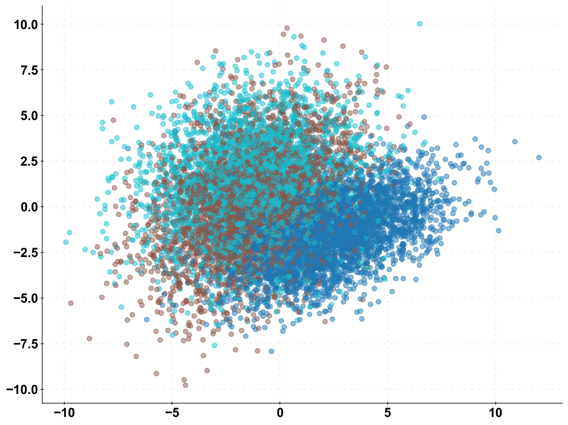
First, we simulate some data with sklearn.datasets.make_classification. To keep it simple, we start of with 3 classes i.e. 3 different possible labels for our data (n_classes = 3). In the plot below, I visualized the data set in 2d-space (after applying PCA) - We do not see a distinct structure and the data just resembles “blobs” in this space.

Second, we split the data into train and test set and estimate two models on the data: A logistic regression model and a very naive “dummy” model. The dummy model makes its prediction based on a random draw i.e. “rolls the dice” on what to predict. We use this “Rolling Dice Model” as a baseline model to compare our hopefully “awesome” logistic regression to.

# generate the data and make predictions with our two models
n_classes = 3

X, y = make_classification(n_samples=10000, n_features=10,
                           n_classes=n_classes, n_clusters_per_class=1,
                           n_informative=10, n_redundant=0)
y = y.astype(int)
X_train, X_test, y_train, y_test = train_test_split(X, y, test_size=0.33, random_state=0)

prediction_naive = np.random.randint(low=0, high=n_classes, size=len(y_test))

clf = LogisticRegression().fit(X_train, y_train)
prediction = clf.predict(X_test)

# take a look at the data in 2d-space
pca = PCA(n_components=2).fit_transform(X)
plt.scatter(pca[:,0], pca[:,1], c=y, cmap=cmap_default, alpha=0.5)
plt.show()

The “Normal” Confusion Matrix

Alright! Now we have our two models and their predictions. Which one should we use for our extremely important fake business case? To give a more refined answer to that, we turn to our confusion matrix. Below, you can see the code that I used to create plots of this matrix.

It consists of two parts: the class CM_Norm and the function plot_cm.

plot_cm computes and visualizes our confusion matrix based on the models prediction (y_pred) and the true values from the test set (y_true). We can also pass it a list of class names to improve the labeling of the matrix. Notice, that we have to normalize the counts in the cells either by the true values or by the predicted values for our graphic to work as intended.

CM_Norm adjusts the diverging colorbar, such that its point of origin is equal to the accuracy expected by chance.
For example: for 3 different classes, the zero of the colorbar would be set at $1/3$.

def plot_cm_standard(y_true, y_pred, list_classes: list, normalize: str, title: str=None, ax=None):
    """ plot the standard confusion matrix!
    :param y_true: np.array, the true values
    :param y_pred: np.array, the predicted values
    :param list_classes: list, of names of the classes
    :param normalize: str, either None, prediction or true
    :param title: str, title of the plot
    """
    import seaborn as sns
    import matplotlib.pyplot as plt
    import numpy as np
    from sklearn.metrics import accuracy_score, confusion_matrix

    # color map and normalization
    cmap = sns.diverging_palette(145, 325, s=200, as_cmap=True)
    norm = CM_Norm(midpoint=1/len(list_classes), vmin=0, vmax=1)

    # the confusion matrix
    cm = confusion_matrix(y_true=y_true, y_pred=y_pred)

    # use normalization?
    if normalize == 'prediction':
        cm = np.round(cm.astype('float') / cm.sum(axis=0)[np.newaxis, :], 2)
    elif normalize == 'true':
        cm = np.round(cm.astype('float') / cm.sum(axis=1)[:, np.newaxis], 2)

    # initialize figure
    #plt.figure()
    ax = sns.heatmap(cm, annot=True, cmap=cmap, square=True, annot_kws={'fontsize':18}, ax=ax, vmin=0, vmax=1)

    # axis labels
    ax.set_xticklabels(list_classes)
    ax.set_yticklabels(list_classes)

    # titles and labels
    accuracy = np.round(accuracy_score(y_true=y_test, y_pred=y_pred), 2)  # compute accuracy
    ax.set_title(title + f" (Acc.: {accuracy})")
    ax.set_ylabel('True')
    ax.set_xlabel('Prediction')

    # layout
    plt.grid(False)
    plt.tight_layout()

class CM_Norm(plt.cm.colors.Normalize):
    """ normalize the colorbar around a value
    """
    def __init__(self, vmin=None, vmax=None, midpoint=None, clip=False):
        self.midpoint = midpoint
        plt.cm.colors.Normalize.__init__(self, vmin, vmax, clip)
    def __call__(self, value, clip=None):
        x, y = [self.vmin, self.midpoint, self.vmax], [0, 0.5, 1]
        return np.ma.masked_array(np.interp(value, x, y), np.isnan(value))

def plot_cm(y_true, y_pred, list_classes: list, normalize: str, title: str=None, ax=None):
    """ plot the confusion matrix and normalize the values
    :param y_true: np.array, the true values
    :param y_pred: np.array, the predicted values
    :param list_classes: list, of names of the classes
    :param normalize: str, either None, prediction or true
    :param title: str, title of the plot
    """
    import seaborn as sns
    import matplotlib.pyplot as plt
    import numpy as np
    from sklearn.metrics import accuracy_score, confusion_matrix

    # color map and normalization
    cmap = sns.diverging_palette(145, 325, s=200, as_cmap=True)
    norm = CM_Norm(midpoint=1/len(list_classes), vmin=0, vmax=1)

    # the confusion matrix
    cm = confusion_matrix(y_true=y_true, y_pred=y_pred)

    # use normalization?
    if normalize == 'prediction':
        cm = np.round(cm.astype('float') / cm.sum(axis=0)[np.newaxis, :], 2)
    elif normalize == 'true':
        cm = np.round(cm.astype('float') / cm.sum(axis=1)[:, np.newaxis], 2)

    # initialize figure
    #plt.figure()
    ax = sns.heatmap(cm, annot=True, cmap=cmap, norm=norm, square=True, annot_kws={'fontsize':18}, ax=ax)

    # axis labels
    ax.set_xticklabels(list_classes)
    ax.set_yticklabels(list_classes)

    # titles and labels
    accuracy = np.round(accuracy_score(y_true=y_test, y_pred=y_pred), 2)  # compute accuracy
    ax.set_title(title + f" (Acc.: {accuracy})")
    ax.set_ylabel('True')
    ax.set_xlabel('Prediction')

    # layout
    plt.grid(False)
    plt.tight_layout()

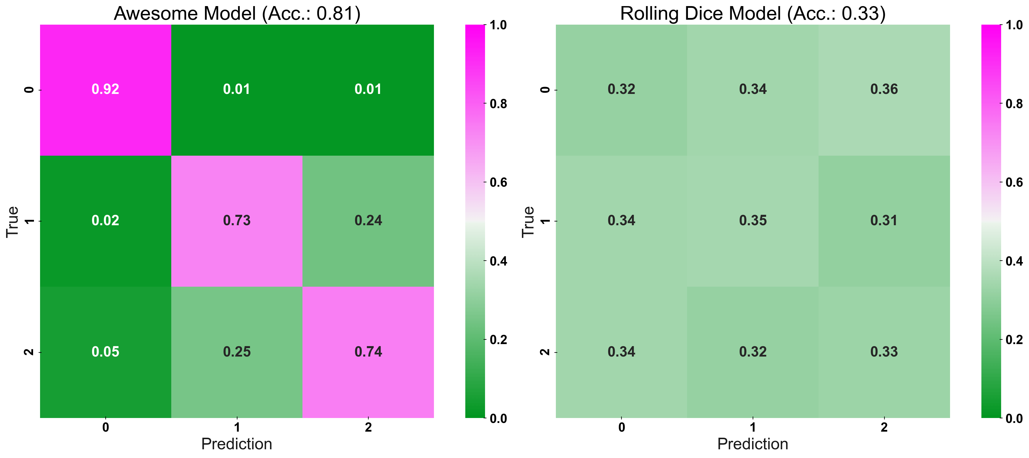
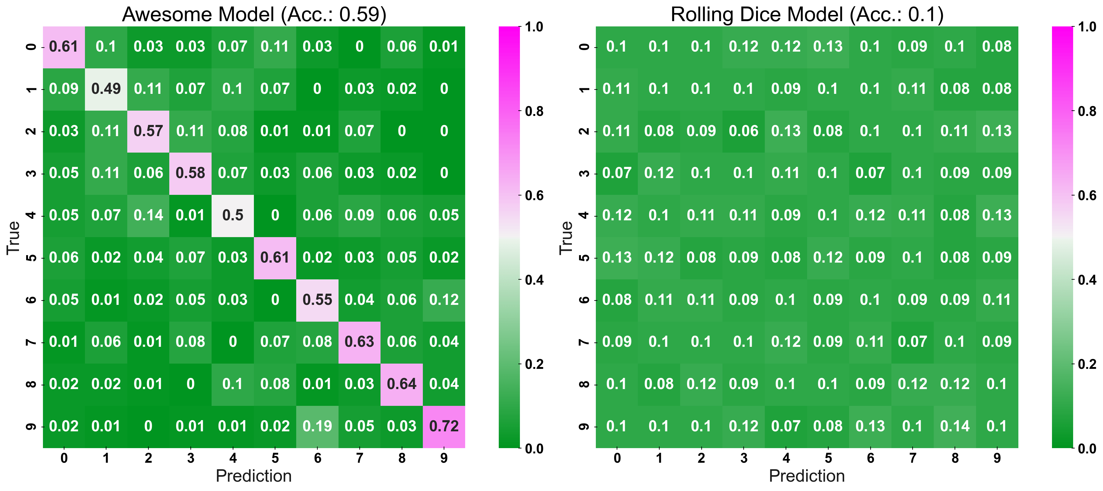
For a first example, I plot the confusion matrix, without paying extra attention to it’s colorbar: We just color cells in accordance to its value. So we have a colorbar with values between 0 and 1. In the following plot, we can see that we at least have a difference in “hue” (i.e. “kind of color” - pink vs. green) for the good model and no difference of main-diagonal and off-diagonal for the bad model.

However, we do not get a very detailed idea of the models properties! 13% are colored as green on the off-diagonal - but is this really and improvement over a naive prediction? What about 40%? It would be colored (light-)green as well, but would actually be worse than by chance!

fig, (ax1, ax2) = plt.subplots(1,2, figsize=(20,8))

plot_cm_standard(y_true=y_test, y_pred=prediction, title="Awesome Model", list_classes=[str(i) for i in range(n_classes)],
        normalize="prediction", ax=ax1)
plot_cm_standard(y_true=y_test, y_pred=prediction_naive, title="Rolling Dice Model", list_classes=[str(i) for i in range(n_classes)],
        normalize="prediction", ax=ax2)
plt.show()

Normalize the Colorbar

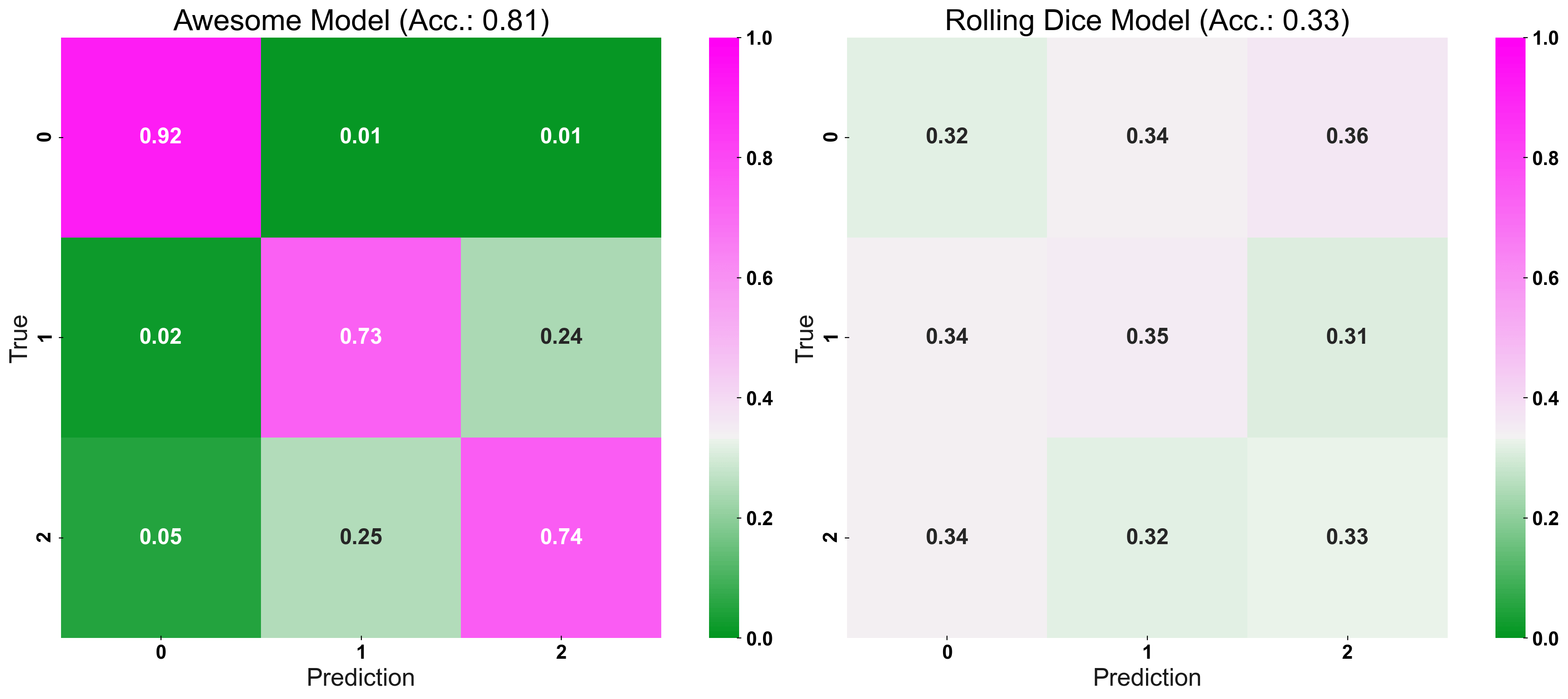
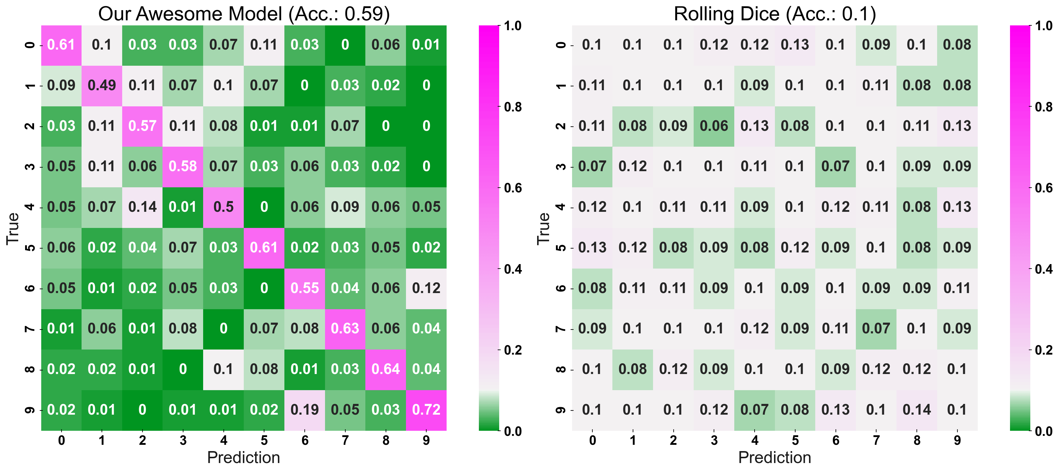
To be able to know at a glimpse, whether our model is performing well or not, the matrice’s cells are color-coded and the colorbar’s point of origin is set to the value anticipated by chance. This leads to more bright colors signaling a worse performance and more dark colors signaling a better performance - regardless of whether we are looking at the main-diagonal (values closer to 1 are better) or one of the off-diagonals (values closer to 0 are better).

Notice that this is more intuitive than just using a not-normalized colorbar: Here, we would need to look at the values in detail and compare them to the performance “anticipated by chance” to make a judgement call — not very intuitive.

In the following plot, we can compare our “Awesome Model” with the “Rolling Dice Model”: The vibrant colors of the “Awesome Model’s” confusion matrix immediately suggest to us its good performance!

Strong colors equal strong model!

fig, (ax1, ax2) = plt.subplots(1,2, figsize=(20,8))

plot_cm(y_true=y_test, y_pred=prediction, title="Awesome Model", list_classes=[str(i) for i in range(n_classes)],
        normalize="prediction", ax=ax1)
plot_cm(y_true=y_test, y_pred=prediction_naive, title="Rolling Dice Model", list_classes=[str(i) for i in range(n_classes)],
        normalize="prediction", ax=ax2)

plt.show()

Create a more Complicated Problem

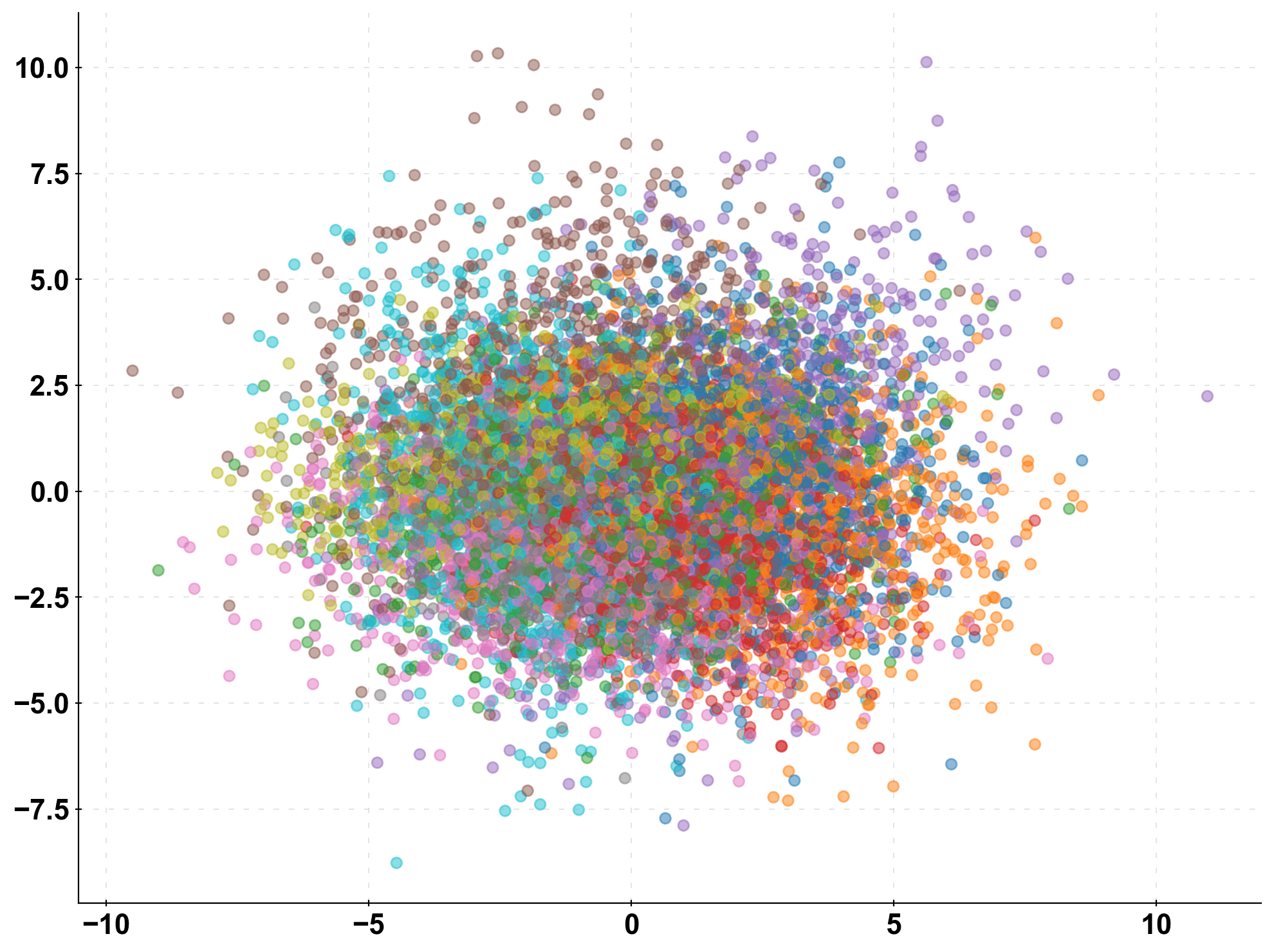
This effect is emphasized if we have even more classes in our classification problem. We repeat the above analysis, but this time with n_classes = 10. Notice, how you can still “glimpse” the models performance even though our problem has gotten way more complicated ($3^2$ cells. vs $10^2$ cells).

n_classes = 10

X, y = make_classification(n_samples=10000, n_features=10,
                           n_classes=n_classes, n_clusters_per_class=1,
                           n_informative=10, n_redundant=0)

X_train, X_test, y_train, y_test = train_test_split(X, y, test_size=0.33, random_state=0)

prediction_naive = np.random.randint(low=0, high=n_classes, size=len(y_test))

clf = LogisticRegression().fit(X_train, y_train)
prediction = clf.predict(X_test)

# take a look at the data in 2d-space
pca = PCA(n_components=2).fit_transform(X)
plt.scatter(pca[:,0], pca[:,1], c=y, cmap=cmap_default, alpha=0.5)
plt.show()

fig, (ax1, ax2) = plt.subplots(1,2, figsize=(20,8))

plot_cm_standard(y_true=y_test, y_pred=prediction, title="Awesome Model", list_classes=[str(i) for i in range(n_classes)],
        normalize="prediction", ax=ax1)
plot_cm_standard(y_true=y_test, y_pred=prediction_naive, title="Rolling Dice Model", list_classes=[str(i) for i in range(n_classes)],
        normalize="prediction", ax=ax2)
plt.show()

fig, (ax1, ax2) = plt.subplots(1,2, figsize=(20,8))

plot_cm(y_true=y_test, y_pred=prediction, title="Our Awesome Model", list_classes=[str(i) for i in range(n_classes)],
        normalize="prediction", ax=ax1)
plot_cm(y_true=y_test, y_pred=prediction_naive, title="Rolling Dice", list_classes=[str(i) for i in range(n_classes)],
        normalize="prediction", ax=ax2)

plt.show()

This wraps it up for this post! I hope you could learn something and find this version of the confusion matrix useful.
Let me know what you think about this article and write me an email to finn@ds-econ.com - I will read every message!