The most simple Machine Learning Pipeline

Code Snippet Repository

Today, we walk thru a basic machine learning pipeline including a train/test split and make use of a random search to conduct a hyperparameter tuning. This architecture is the backbone of many statistical machine learning tasks and hence usefuls as to keep close-by as a code-snippet!

# load modules and get a data set
import pandas as pd
import seaborn as sns
import matplotlib.pyplot as plt
from sklearn.datasets import make_classification

X, y = make_classification(n_samples=1000)  # generate a class. problem

# ds-econ style sheet!
plt.style.use('/Users/hoener/Documents/ds-econ/dev/src/ds_econ_stylesheet')
cmap_default = sns.color_palette("tab10", as_cmap=True)

The Basic Machine Learning Pipeline

The first step in our mini “pipeline” is to split the data set into training and test set. This splitting of the data is important, to prevent overfitting and have an evaluation of the model which reprensents its real-life performance more closely. We can do this in a neat way with sklearn’s model_selection.train_test_split.

from sklearn.model_selection import train_test_split

# create train-test split
X_train, X_test, y_train, y_test = train_test_split(
    X, y, test_size=0.25, random_state=0)

Next, we initialize our model. We use sklearn’s linear_model.LogisticRegression here, but choice is arbitrary for this example.
Go take a look at the documentation of scikit-learn, for information on all models and other useful machine learning functions contained in this seminal package!

We initialize the model with fixed hyperparameters, fit it to the training data (i.e. X_train & y_train) and then we make a prediction with the model on the test data i.e. X_test. Below, we then use the labels of the test set (y_test) to evaluate the models performance with metrics.accuaracy_score.

Note: the test set is not used to train the model - It is used to evaluate it!

# train the model on the training data
from sklearn.linear_model import LogisticRegression

# initialize the model with fixed hyperparameters - see doc!
model = LogisticRegression(penalty="l2", C=1.0, random_state=0)

# fit the model to the data
model.fit(X_train, y_train)

# make a prediction on unseen data i.e. the test set
prediction = model.predict(X_test)

from sklearn.metrics import accuracy_score
# calculate the performance as the accuracy score
print(f'The models accuracy is: {accuracy_score(y_test, prediction)}')

The models accuracy is: 0.904

Getting More Complex: Adding Hyperparameter-Tuning

After walking through the example code above, you might have asked yourself: “How do we pick the hyperparameters though?”. While there are general rules-of-thumb for some algorithm’s hyperparameters out there, a good appraoch in either case is to make use of Hyperparameter-Tuning with Cross-Validation. You can read more about this topic in this Towards-Data-Science Article

In this example we use RandomizedSearchCV, which randomly chooses configurations of hyperparameters out of a prespecified set (the dictionary: dist_param). You can read more about the details of this function in its documentation.

For this second part, we use a different model just to switch things up. Here, we use a Decision-Tree: DecisionTreeClassifier.

from sklearn.model_selection import train_test_split

# create train-test split
X_train, X_test, y_train, y_test = train_test_split(
    X, y, test_size=0.25, random_state=1)

from scipy.stats import norm

# initilaize RandomSearch
dist_param = {'max_depth':[1, 5, 10, 20], 'criterion':['gini', 'entropy']}

To conduct the RandomizedSearchCV, we first specify the type of model we want to use and pass any hyperparameters that we want to fix for it here. In a second step, we pass this model into RandomizedSearchCV and fix some options of the cross-validation, like the number of cv-splits or which random_state to use.

# train the model on the training data
from sklearn.tree import DecisionTreeClassifier
from sklearn.model_selection import RandomizedSearchCV

model = DecisionTreeClassifier(random_state=0)
rcv = RandomizedSearchCV(model, dist_param, random_state=1, verbose=3, n_iter=5, 
                         cv=3)

# fit the model to the data
rcv.fit(X_train, y_train)

# make a prediction on unseen data i.e. the test set
prediction = rcv.predict(X_test)

Fitting 3 folds for each of 5 candidates, totalling 15 fits
[CV 1/3] END ...criterion=entropy, max_depth=20;, score=0.924 total time=   0.0s
[CV 2/3] END ...criterion=entropy, max_depth=20;, score=0.920 total time=   0.0s
[CV 3/3] END ...criterion=entropy, max_depth=20;, score=0.928 total time=   0.0s
[CV 1/3] END ......criterion=gini, max_depth=10;, score=0.932 total time=   0.0s
[CV 2/3] END ......criterion=gini, max_depth=10;, score=0.924 total time=   0.0s
[CV 3/3] END ......criterion=gini, max_depth=10;, score=0.948 total time=   0.0s
[CV 1/3] END .......criterion=gini, max_depth=5;, score=0.944 total time=   0.0s
[CV 2/3] END .......criterion=gini, max_depth=5;, score=0.944 total time=   0.0s
[CV 3/3] END .......criterion=gini, max_depth=5;, score=0.960 total time=   0.0s
[CV 1/3] END ...criterion=entropy, max_depth=10;, score=0.924 total time=   0.0s
[CV 2/3] END ...criterion=entropy, max_depth=10;, score=0.920 total time=   0.0s
[CV 3/3] END ...criterion=entropy, max_depth=10;, score=0.928 total time=   0.0s
[CV 1/3] END .......criterion=gini, max_depth=1;, score=0.924 total time=   0.0s
[CV 2/3] END .......criterion=gini, max_depth=1;, score=0.912 total time=   0.0s
[CV 3/3] END .......criterion=gini, max_depth=1;, score=0.916 total time=   0.0s

Great! In the output above, we get a glimpse into the tuning process: The random search draws 5 combinations (n_iter=5) of hyperparameters and evaluates each of these combinations in a 3 fold cross-validation (cv=3). The configuration with the best score is then selected for the model and used to fit it on the whole training set. Here, criterion=gini and max_depth=5 is the most potent configuration with an accuracy of $ 96% $.

This tuned decision-tree performsbetter than the one of the untuned logistic regression on the test set (see below).

from sklearn.metrics import accuracy_score
# calculate the performance as the accuracy score
print(f'The models accuracy is: {accuracy_score(y_test, prediction)}')

The models accuracy is: 0.944

Using the Optimal Hyperparameters in a different Model

We can also extract these optimal hyperparameters to specify them directly in our model. This extraction can be useful, if we want to use the model for adjacent purposes like for example visualizing a decision-tree in a graph.

See below for the implementations of the hyperparameters extraction and the final plot of the decision tree!

best_params = rcv.best_params_  # get the best hyperparameters found by RS
print(best_params)

{'max_depth': 5, 'criterion': 'gini'}

Note how we need to unlist the dictioanry best_params by prefixing it with **best_params!

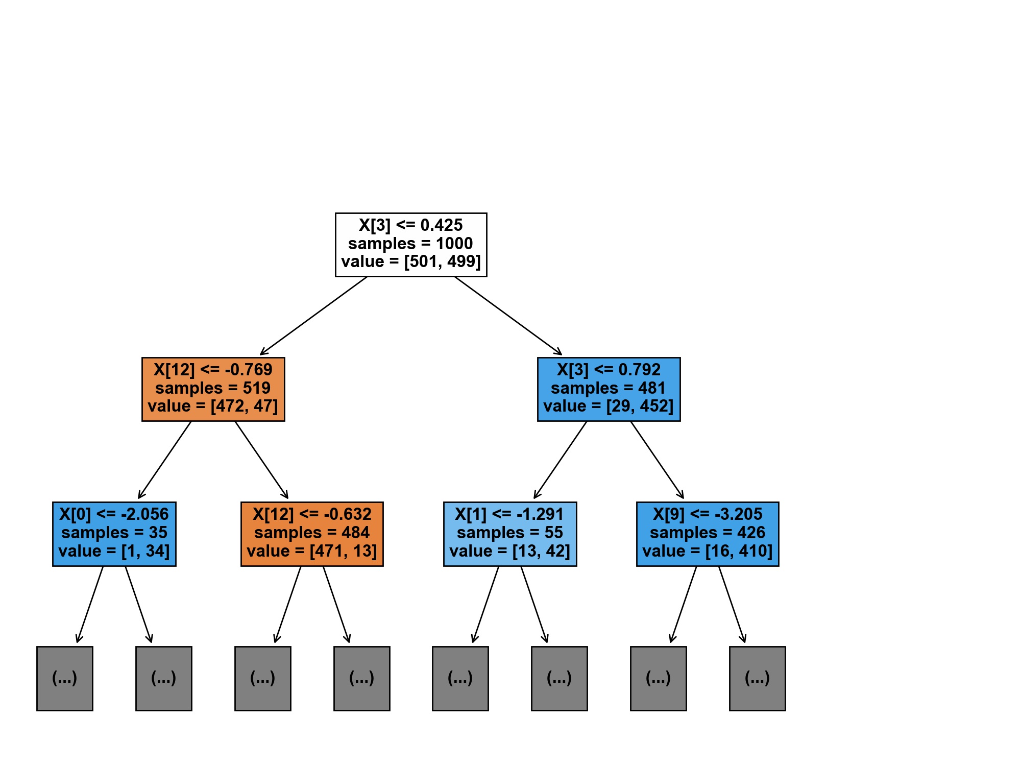
Finally, we make use of plot_tree to visualize our Decision-Tree below! Usually, we could try to interpret it and try to get a better intution for what our model is doing, however this does not make a lot of sense with simulated data.

from sklearn.tree import plot_tree

# plot the decision tree for better intuition
model_tree = DecisionTreeClassifier(**best_params)  # unpack the dictionary

model_tree.fit(X, y)  # fit on whole data set for the plot

# plot the decision tree with plot_tree
fig, axes = plt.subplots(nrows = 1,ncols = 1,figsize = (10,7.5), dpi=200)
plot_tree(model_tree, impurity=False, ax=axes, filled=True, max_depth=2,
          fontsize=12)

plt.close()

Code Snippet Repository

This post is part of the Code Snippet Repository, a collection of short posts designed to make your everyday coding easier. These are based on public content from forums like stackoverflow and package documentations. You can find the code also in this repo on github!

Photo by Simon Wilkes on Unsplash